Keywords: TGA, DSC, Curve Fitting, Deconvolution, Pearson IV, peak deconvolution, chemometrics
TA431
Abstract
Overlapping thermal transitions observed in TGA and DSC experiments can be resolved to varying levels of success using numerical deconvolution methods. In this work, we demonstrate deconvolution with two examples of thermal data fitted using some commonly cited mathematical models used for deconvolution of asymmetric and tailing data. Despite good quality of the data fit, there is significant scatter in the calculated results depending on the model chosen, so independent assessment of the bias of the analysis is necessary.
Introduction
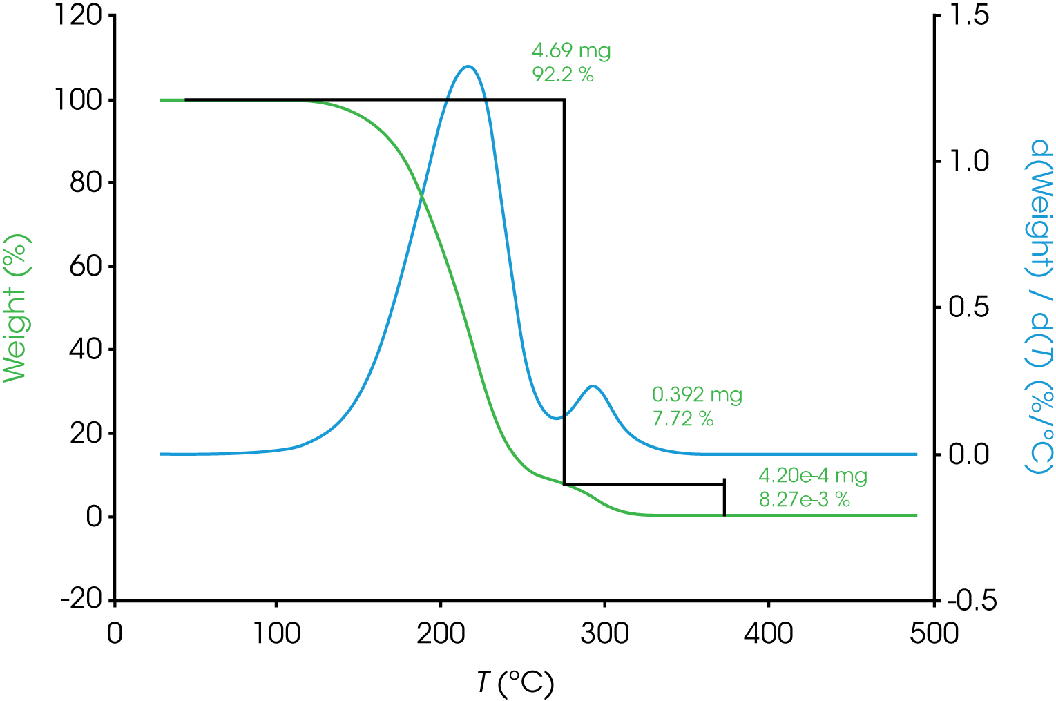
Overlapping transitions like those sometimes encountered in spectroscopy and chromatography data are also common in thermal analysis data. Consider the TGA data shown in Figure 1 of the mass loss of an engine oil ‘A’. The oil shows two apparent single step changes in mass. The relative symmetry of the derivative curves (shown in blue) are a good indicator of two monotonous mass losses although it is a subjective observation. A common approach to analyzing TGA mass loss data is to use the local minimum in the derivative curve as a guide for choosing the analysis limits. In the example shown in Figure 1 a result of 92% for the first mass loss, 8% for the second, and a negligible amount of residue was obtained. When the derivative curve is well resolved as in the case of engine oil ‘A’, good precision can be expected assuming consistency choosing limits.
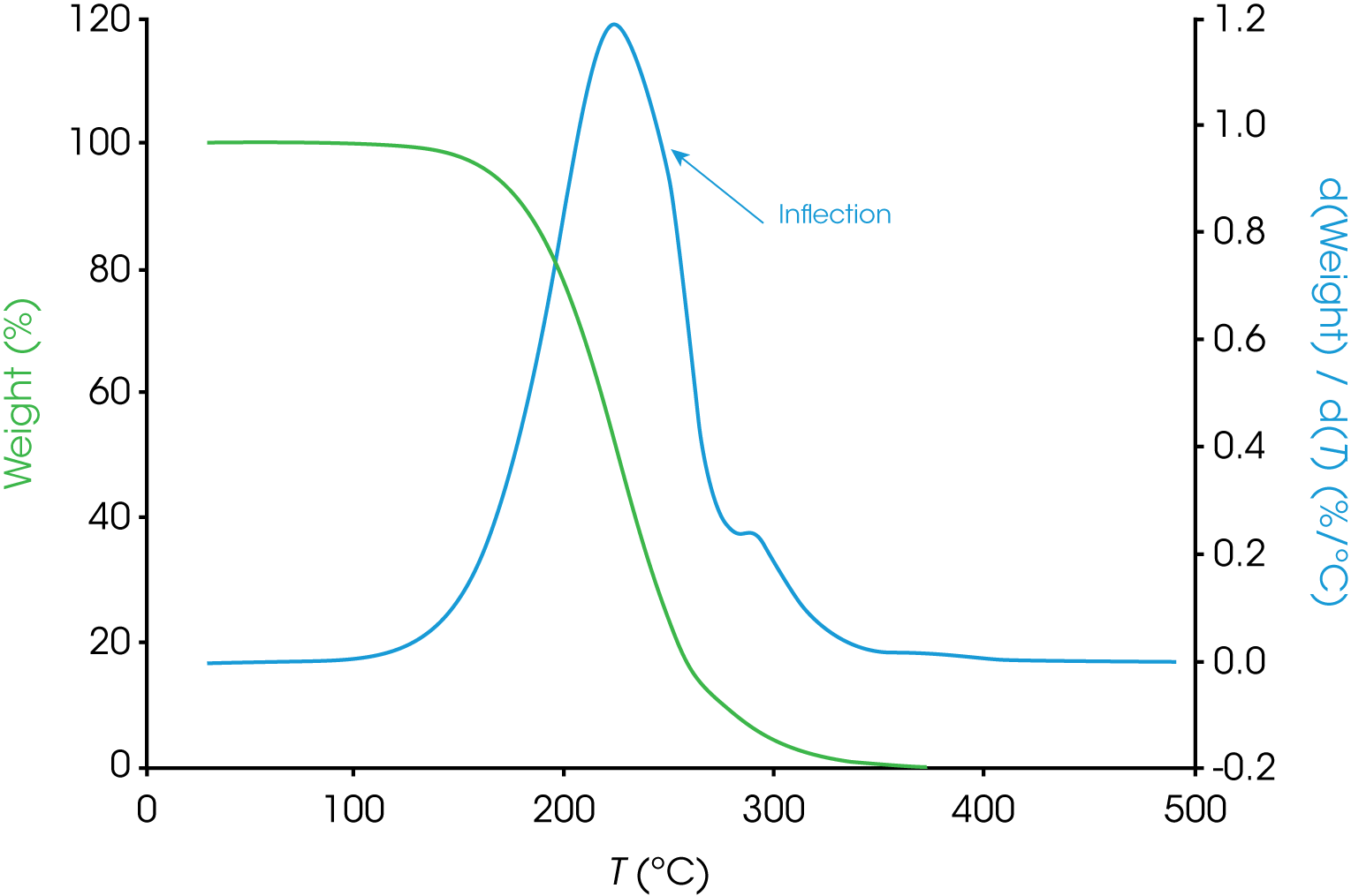
The analysis for engine oil ‘B’ shown in Figure 2 is not straightforward. Notice the inflection in the derivative curve. One simple interpretation is that the inflection is due to different rates of mass loss caused by different decomposition kinetics in this first mass loss event. This may imply the presence of more than one component, interaction of two components, possible transformation of one component into a form with different decomposition kinetics, etc. Estimating the beginning of the smaller transition centered around 300 °C is also not as simple in oil ‘B’.
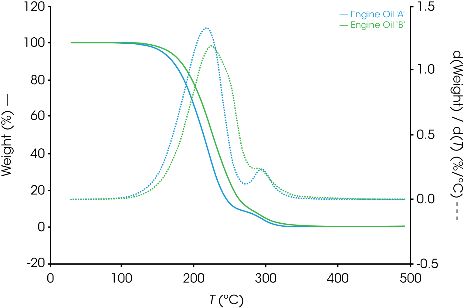
The differences in between oils A and B are more apparent when the mass loss derivatives are overlaid in Figure 3.
One approach to analyze overlapping transitions is to apply a deconvolution method to the data to determine the relative area contribution of the components.
In the case of TGA, the mass loss data is the summation or integral of the decomposition by way of mass loss of the components present, so the derivative with respect to either time or temperature serves as the function for deconvolution.
In the case of DSC data, this is simply the heat flow curve which is a differential (Equation 1)

Where dq/dt is the differential heat flow rate, CP is the specific heat capacity, dT/dt is the heating rate (sometimes abbreviated as β), and f(T,t) are temperature and time dependent functions. A complication of deconvolution of DSC data is the possibility of simultaneous endothermic and exothermic transitions often prevalent in polymorphic transformations as an example. Careful evaluation of these potential kinetic dependent transitions should be undertaken before attempting any deconvolution.
Background
The problem of resolving overlapping peaks is certainly not new. Asymmetry, significant fronting, and sometimes tailing often observed in thermal data results in distributions that are not modeled ideally with Gaussian or Lorentzian functions often used to deconvolve spectroscopic and chromatographic data. Several approaches have been published in the literature using functions that fit asymmetric data. Koga and coworkers [1] fit TGA data using 9 different mathematical functions including asymmetric double sigmoid, asymmetric logistic, extreme value 4 parameter fronted, Fraser-Suzuki, log normal 4 parameter, logistic power peak, Pearson IV, Pearson IV (a3 = 2), and Weibull with fitting criterion that r2 > 0.99.
Michael et al. developed a function for deconvolving DSC nickel titanium phase transformation heat flow data [2]. Deconvolution has been used to separate complex chemical processes for kinetic analysis shown in Figure 4 by Khachani et al. [3]
For this work, we fit examples using the following models: Pearson IV, Asymmetric Logistic, Extreme Value 4 Parameter Fronted, Log Normal 4 Area, Logistic Power Peak, and Exponentially Modified Gaussian (EMG).
![TA431_Fig.4 Figure 4. Peak Deconvolution Using Frazer-Suzuki Function; β=7 °C/min [3]](https://www.tainstruments.com/wp-content/uploads/TA431_Fig.4.png)
Experimental
- Example 1 – Comparison of Two Motor Oils
a. Instrument – TA Instruments Discovery 5500 TGA
b. Heating Rate 1 °C / min (modulated TGA Experiment)
c. Crucible – Pt
d. Purge – N2 at 25 mL / min
e. Sample Mass – 5 mg nominal - Example 2 – Dynamic Curing of Epoxy
a. Instrument – TA Instruments Discovery 2500 DSC
b. Heating Rate – 10 °C / min
c. Purge – N2 at 50 mL / min
d. Crucible – Tzero Aluminum
e. Sample Mass – 2 mg nominal
Data Reduction
TGA and DSC data were exported as text files and analyzed using PeakFit v4.12 (Systat). The models used for fitting the data are contained in the software. For conciseness, we show illustrated data only from the Pearson IV fit.
Results and Discussion
1. Comparison of Two Motor Oils
a. Oil ‘A’ – Figure 5 (same data as Figure 1) shows a typical TGA data reduction for this sample. The limits chosen where based on the position of the relative minima of the derivative curves.
Figure 6 shows the deconvolution of the derivative of mass loss with respect to temperature signal using the Pearson IV model. Other models and the resultant area fractions are summarized in Table 1
Residuals for Oil ‘A’ are shown in Figure 7
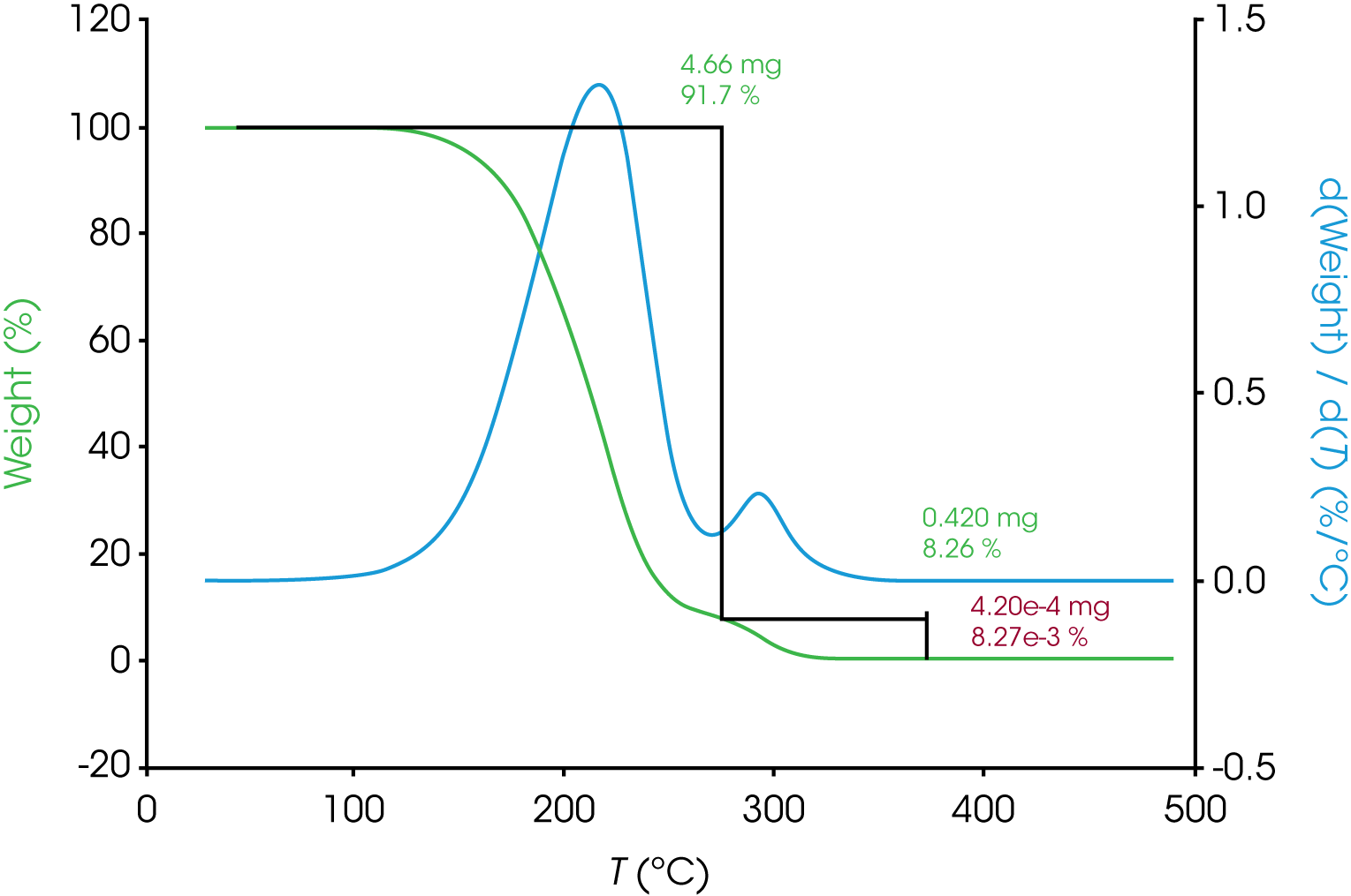
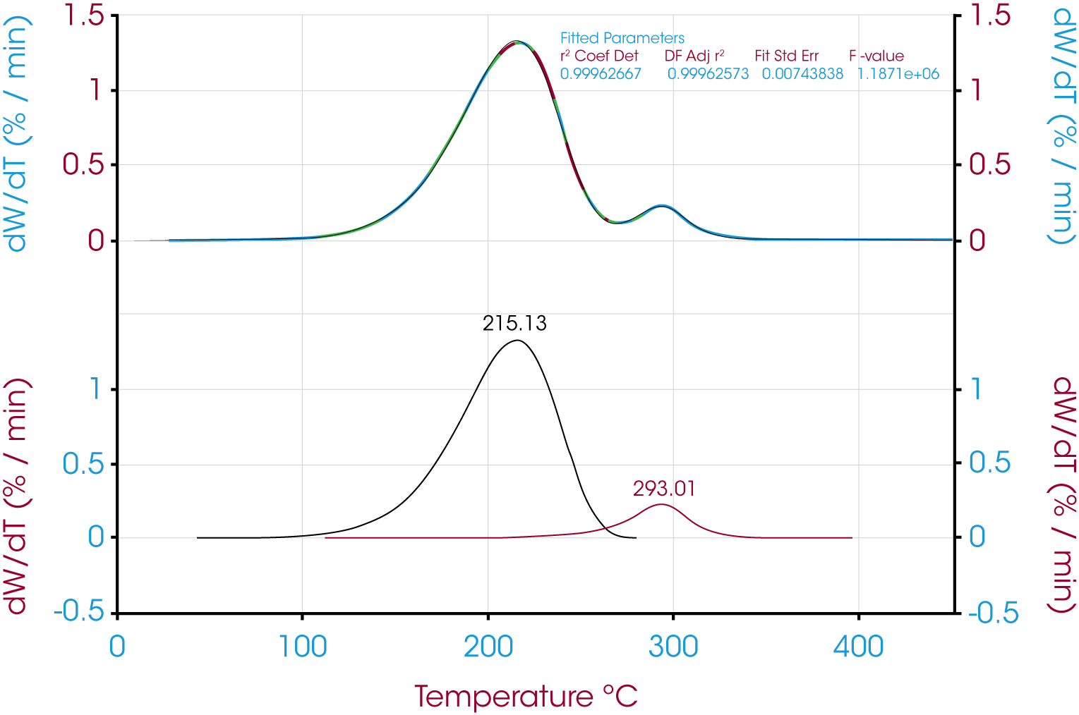
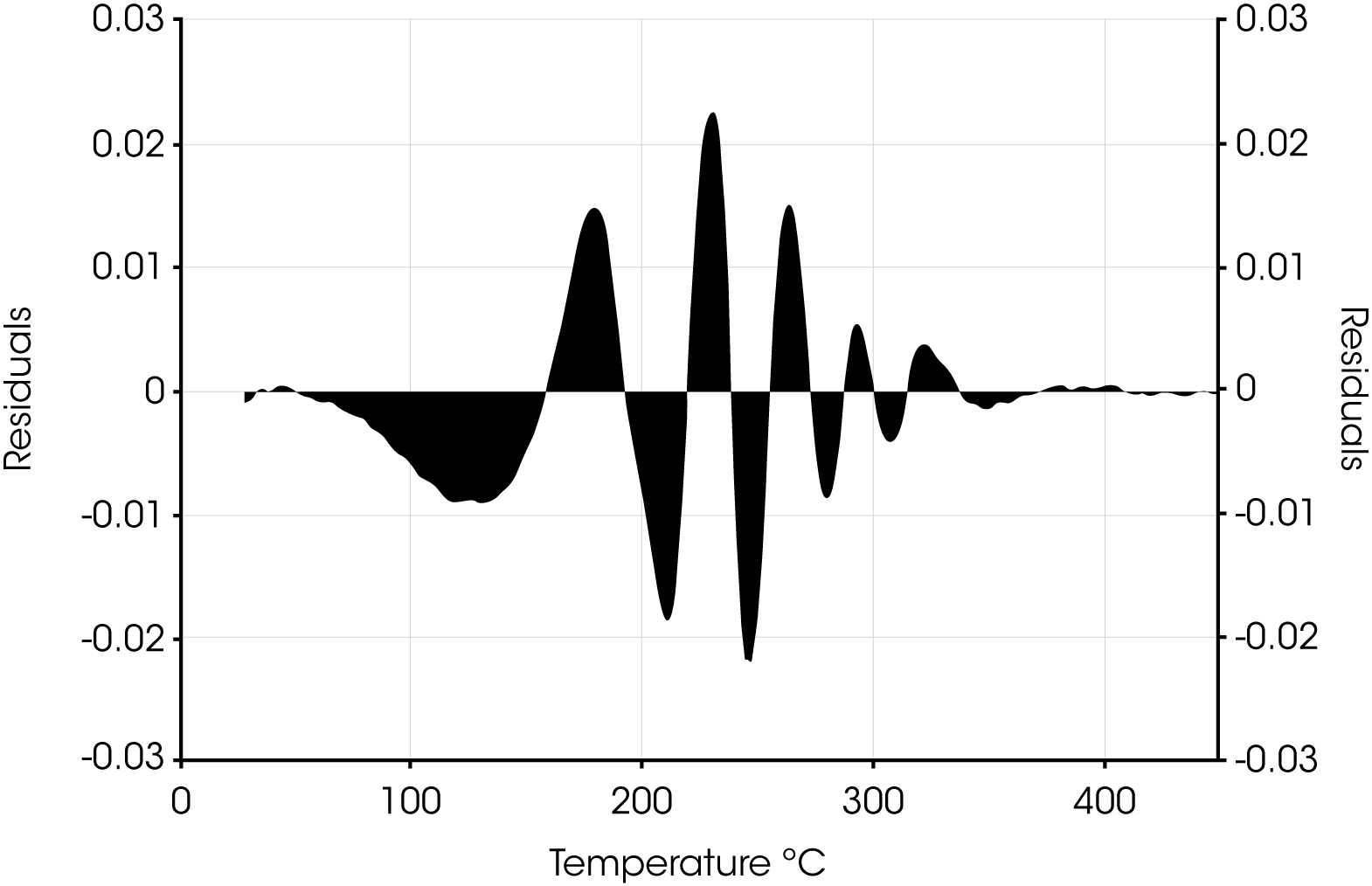
Table 1. Area % Calculations for Oil ‘A’ by Model
| Model | Peak 1 % | Peak 2 % | r2 | Standard Error |
|---|---|---|---|---|
| Pearson IV | 89.37 | 10.63 | 1.000 | 0.0072 |
| Asymmetric Logistic | 93.30 | 6.70 | 0.997 | 0.0202 |
| Extreme Value 4 Area Fronted | 91.12 | 8.884 | 0.999 | 0.0084 |
| Log Normal-4-Area | 90.82 | 9.179 | 1.000 | 0.0079 |
| Logistic Power Peak | 93.38 | 6.622 | 0.997 | 0.0211 |
| Exponentially Modified Gaussian | 92.06 | 7.94 | 0.998 | 0.0154 |
| Derivative Minimum | 91.7 | 8.26 | – | – |
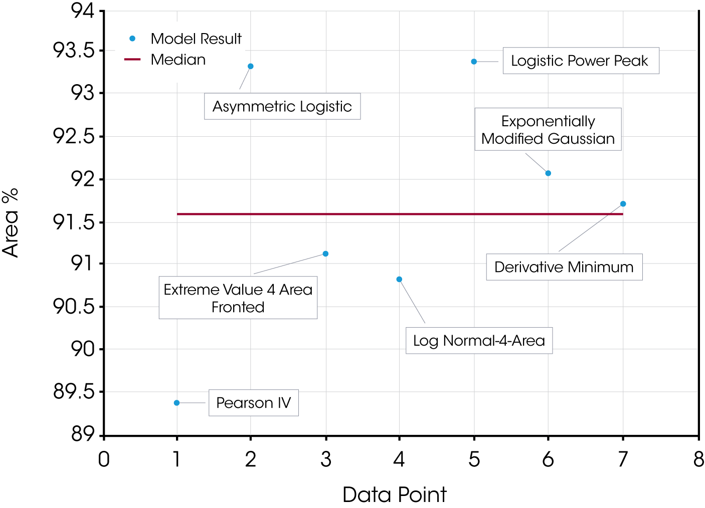
The quality of the data fit using the models is good but in this case the results obtained using the using the derivative minimum as a guideline lie withing the scatter range of the results obtained using the models. This is explained by the relatively good separation of the mass loss events. The scatter of the data set is shown in Figure 8.
b. Oil ‘B’ – Figure 9 (same data as Figure 2) shows the data reduction for this sample. As stated previously, the first mass loss does not appear to be monotonous and deconvolution should make improvements to more accurately analyze the data.
Figure 10 shows the deconvolution of the derivative of mass loss with respect to temperature using the Pearson IV model.
Residuals for Oil ‘B’ are shown in Figure 11.
Table 2 compares area fraction differences in oil sample ‘B’ using the models and the derivative minimum method.
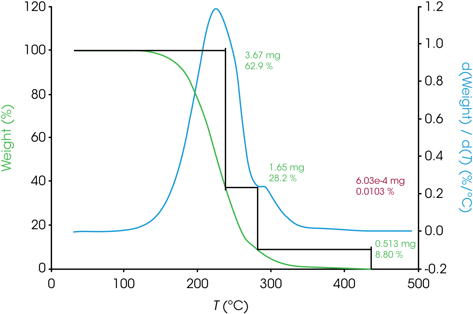
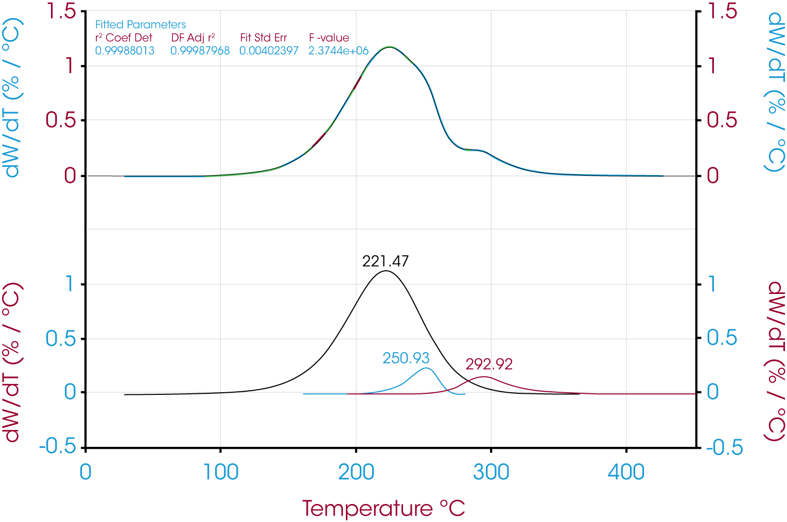
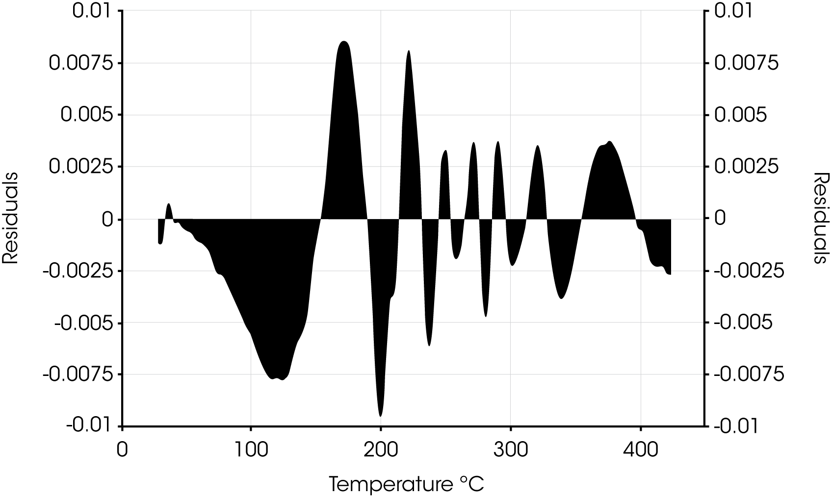
Table 2. Area % Calculations for Oil ‘B’ by Model
| Model | Peak 1 % | Peak 2 % | Peak 3 % | r2 | Standard Error |
|---|---|---|---|---|---|
| Pearson IV | 84.83 | 7.04 | 8.13 | 1.000 | 0.0040 |
| Asymmetric Logistic | 83.63 | 8.61 | 7.76 | 0.999 | 0.0107 |
| Extreme Value 4 Area Fronted | 79.16 | 7.55 | 13.29 | 1.000 | 0.0081 |
| Log Normal-4-Area | 82.25 | 6.11 | 11.64 | 1.000 | 0.0034 |
| Logistic Power Peak | 87.52 | 6.01 | 6.47 | 1.000 | 0.0060 |
| Exponentially Modified Gaussian | 83.82 | 6.46 | 9.72 | 1.000 | 0.0070 |
| Derivative Minimum | 62.9 | 28.2 | 8.80 | – | – |
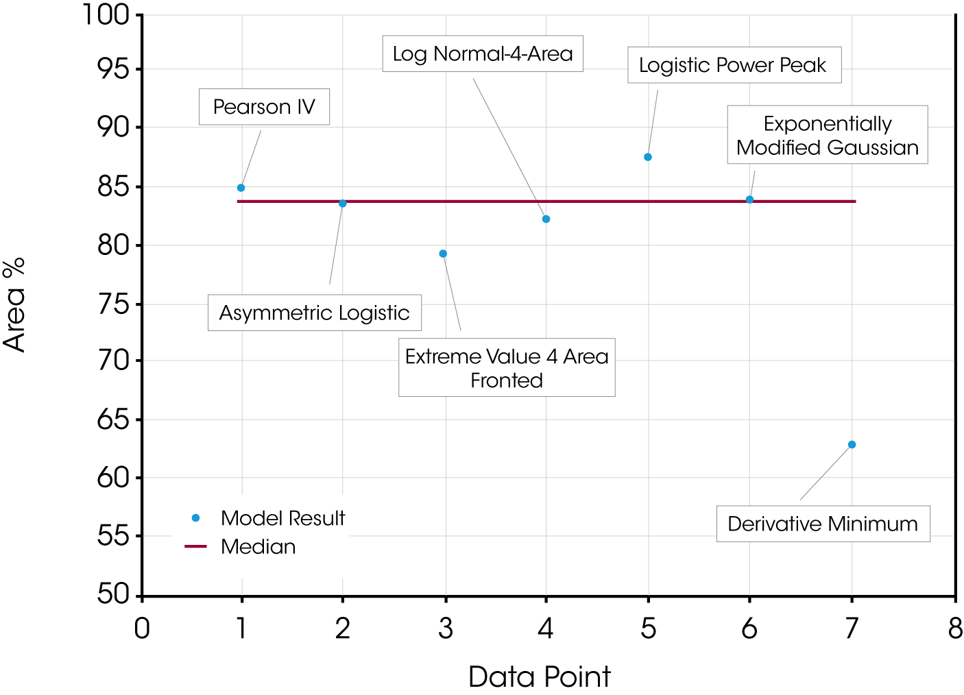
In this case the quality of the data fit is also good and likely does improve the accuracy of the data relative to the derivative minimum. There is also significant scatter within the results obtained using the models and is shown in Figure 12.
2. DSC Evaluation of Epoxy Curing – This example shows two dynamic temperature ramps of a common epoxy. At time t0, the DSC analysis is straightforward and is shown in Figure 13.
At time t as the epoxy cures, a second diffusion driven exothermic transition becomes apparent shown in Figure 14.


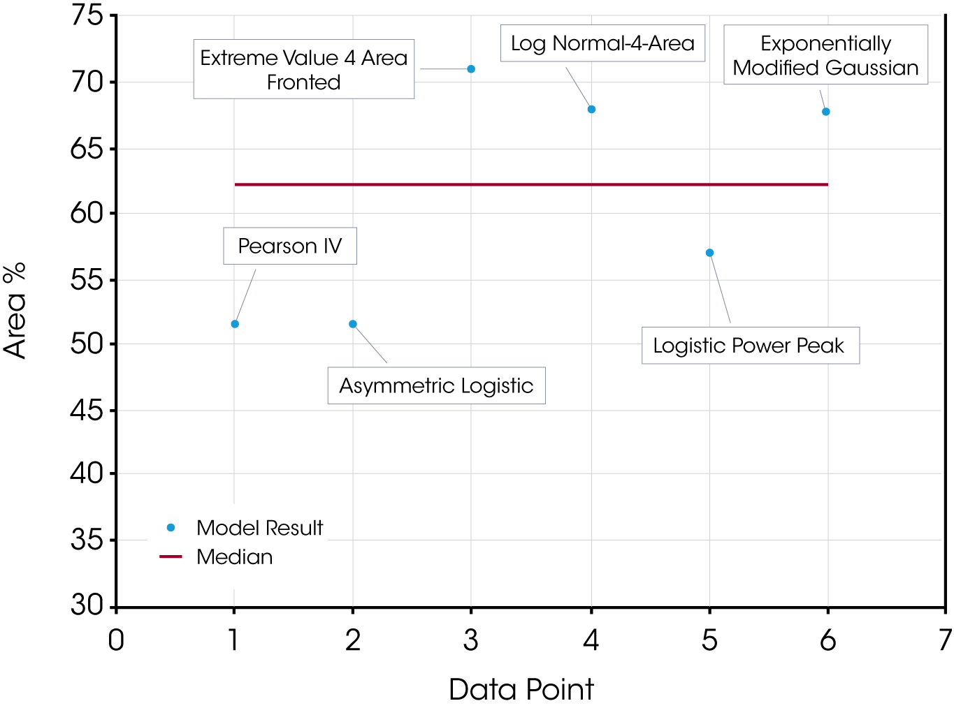
In this case where the peaks are poorly resolved, deconvolution is a means to a more accurate value for the relative contribution of the reaction and diffusion heat flow. Deconvolution of the epoxy at time t shown in Figure 15 and residuals are shown in Figure 16.
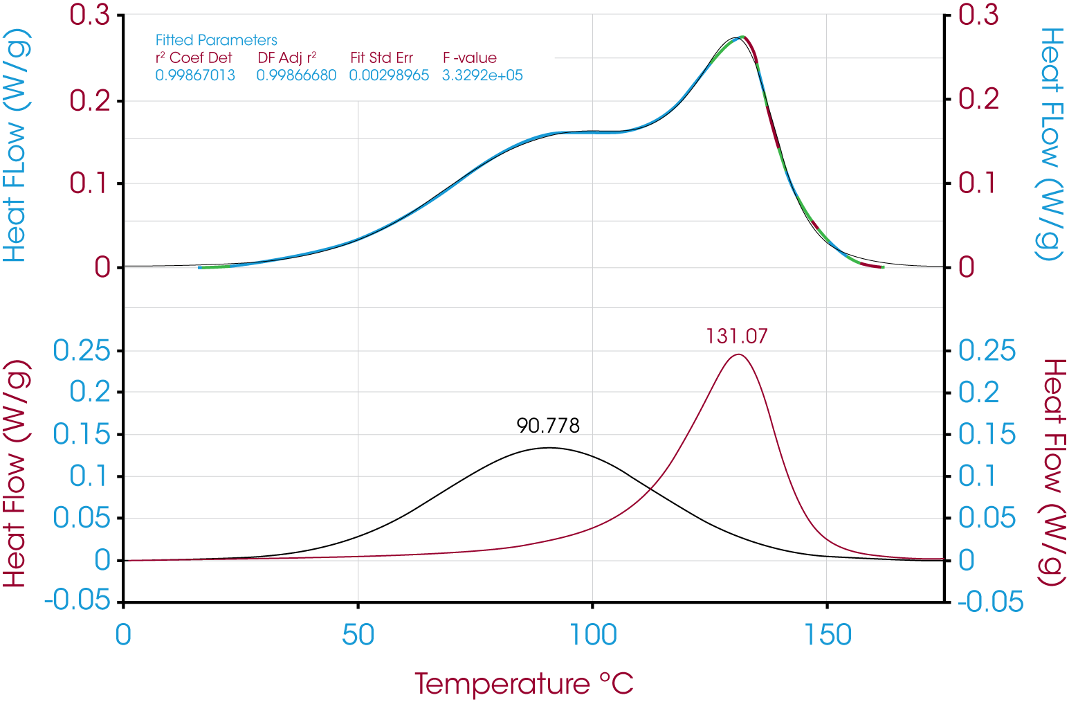

Table 3 summarizes and compares the relative peak areas of the reaction and diffusion heat flow due to the curing of the epoxy.
The quality of the data fit using the models in this example is also good and likely approaches accurate results. We expect that the uncertainty in this particular example would be partially mitigated by choosing fit parameters for the reaction (1st exotherm) and diffusion exotherms (2nd exotherm) based on the apparent symmetry of the reaction exotherm at time t0 assuming that the corresponding reaction exotherm at time t (Figure 14) is similar. Despite the advantage of obtaining the t0 data, the models yield significantly different values. Scatter of the first peak of the epoxy data is shown in Figure 17. The choice of the initial fitting parameters is subjective, but the PeakFit software makes this easy with an interactive interface. A derivative minimum approach was not attempted for this sample.
Table 3. Area % Calculations for Partially Cured Epoxy by Model
| Model | Peak 1 % | Peak 2 % | r2 | Standard Error |
|---|---|---|---|---|
| Pearson IV | 51.42 | 48.58 | 0.999 | 0.0030 |
| Asymmetric Logistic | 51.60 | 48.40 | 0.998 | 0.0032 |
| Extreme Value 4 Area Fronted | 71.15 | 28.85 | 0.997 | 0.0044 |
| Log Normal-4-Area | 67.79 | 32.21 | 0.997 | 0.0045 |
| Logistic Power Peak | 56.93 | 43.07 | 0.997 | 0.0046 |
| Exponentially Modified Gaussian | 67.72 | 32.28 | 0.997 | 0.0038 |
| Derivative Minimum | 62.9 | 28.2 | 8.80 | – |
Conclusions
Peak deconvolution is a practical tool to determine a more accurate relative contribution of unresolved thermal analysis events and is often used to resolve spectroscopic and chromatographic data. The mathematical models used for deconvolution in our examples show good correlation and standard error, but also show considerable scatter so that it is difficult to determine which yields the most accurate result. Independent assessment of the bias and error of the utilized model is needed especially in the user’s choice of initial fitting parameters.
We used the same model for fitting each of the peaks in the examples and this may be a good starting point but is likely too simplistic an approach.
References
- Koga, N., Goshi, Y., Yamada, S., Perez-Maqueda, L.; Kinetic Approach to Partially Overlapped Thermal Decomposition Processes; J Thermal Analytical Calorimetry (2013) 111:1463–1474
- Michael, A., Zhou, Z., Yavuz, M., Khan, M.; Deconvolution of Overlapping Peaks from Differential Scanning Calorimetry Analysis for Multi-Phase NiTi Alloys; Thermochimica Acta 665(2018) 53-59
- Khachani, M., Hamidi, A., et al; Kinetic Approach of Multi-Step Thermal Decomposition Processes of Iron(III) Phosphate Dihydrate (FePO4.2H2O); Thermochimica Acta 610 (2015) 29-36
- Heinrich, J.; A Guide to the Pearson Type IV Distribution; The Collider Detector and Fermilab Website Notes on Statistics; https://www cdf.fnal.gov/physics/statistics/notes/cdf6820_ pearson4.pdf
- Wang, T., Arbestain, M., Hedley, M., Singh, B., Pereira, R., Wang, C.; Determination of Carbonate-C in Biochars; Soil Research, 2014, 52, 495–504, http://dx.doi.org/10.1071/SR13177
- QL Yan, Zeman, S., et al.; Multi-stage Decomposition of 5- aminotetrazole Derivatives: Kinetics and Reaction Channels for the Rate-limiting Steps; Phys.Chem.Chem.Phys., 2014, 16, 24282
- Leitao, M., Canotilho, J.,Cruz, M., Pereira, J., Sousa, A., Redinha, J.; Study of Polymorphism from DSC Melting Curves – Polymorphs of Terfenadine; Journal of Thermal Analysis and Calorimetry, Vol 68 (2002) 397-412
- Carbon Component Estimation with TGA and Mixture Modeling; https://smwindecker.github.io/mixchar/articles/Background.html
- Zhao, S.F., et al. Curing Kinetics, Mechanism and Chemorheological Behavior of Methanol Etherified Amino /Novolac Epoxy Systems; Polymer Letters Vol.8, No.2 (2014) 95–106
Acknowledgement
Gray Slough, Ph.D., Product Marketing Specialist at TA Instruments.
Click here to download the printable version of this application note.

