Keywords: DSC, modeling, baseline, biomolecules, pharmaceuticals
MC154
Introduction
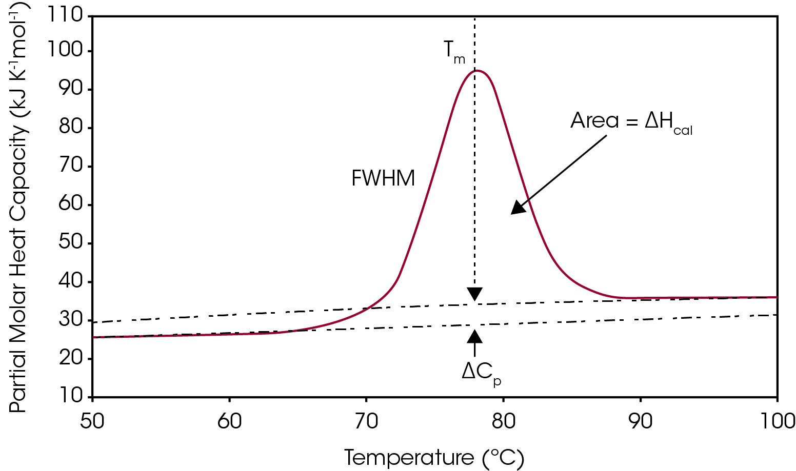
One way to analyze the stability of a macromolecule in dilute solution is to determine the changes in the partial molar heat capacity of the macromolecule at constant pressure (ΔCp). The change in the heat capacity of a compound reflects its ability to absorb heat and experience a defined increase in temperature. During the unfolding process not only is the macromolecule denaturing (breaking of hydrogen bonds and disruption of hydrophobic interactions),1 but the water molecules also begin to restructure as more non-polar sidechains are exposed.2-3 This is what leads to a shift in the baseline as there is a change in the heat capacity when going from the native to unfolded structure, shown in Figure 1. The other parameters from a typical DSC curve are TM, which is the temperature at which half the macromolecules are folded, and the other half unfolded. The integration of the transition reflects ΔHcal, the enthalpy measured directly from the Nano DSC during the unfolding event. Finally, the full width half max (FWHM) value can be determined, which can be used to compare cooperativity between different samples. There is a lot of information that can be obtained directly from the analysis curve without needing to model the data, however, choosing to model DSC data can give additional insight into the unfolding process of a macromolecule or be helpful to deconvolute a multiple transition thermogram. This application note will discuss general guidelines of choosing the correct baseline and DSC model.
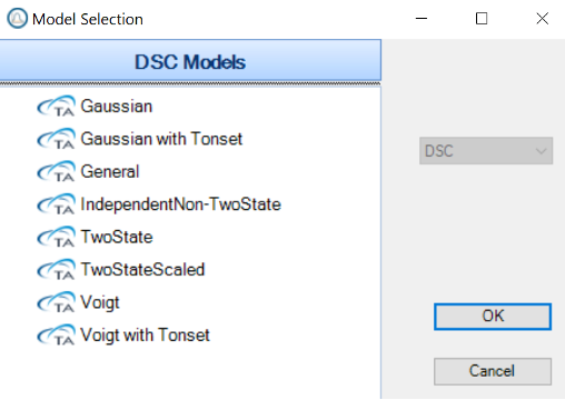
That said, there are many scenarios when it comes to fitting DSC data, so in this application note we will only cover a few basic data sets. Within the NanoAnalyze software there are 5 sets of models, shown in Figure 2. Now, it is important to note there are times where one could choose from multiple models and still be correct. So, it is important to be consistent on the model type that is chosen when more than one could apply. This allows for better direct comparison of data between samples.
Discussion
Baseline Construction
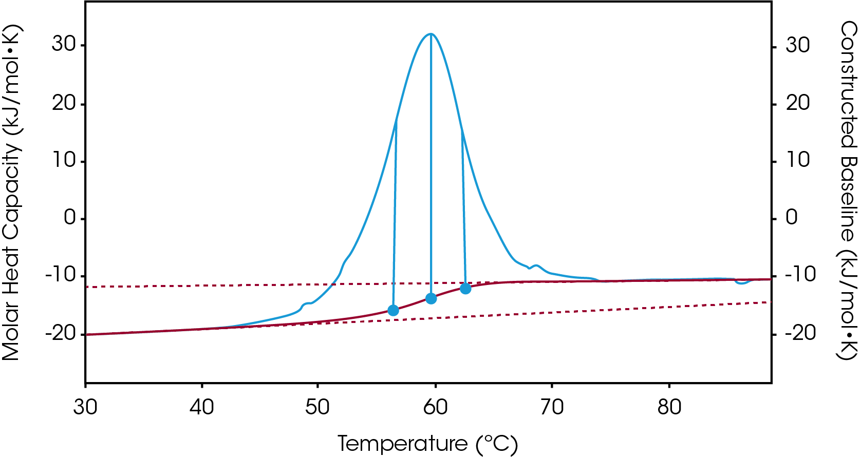
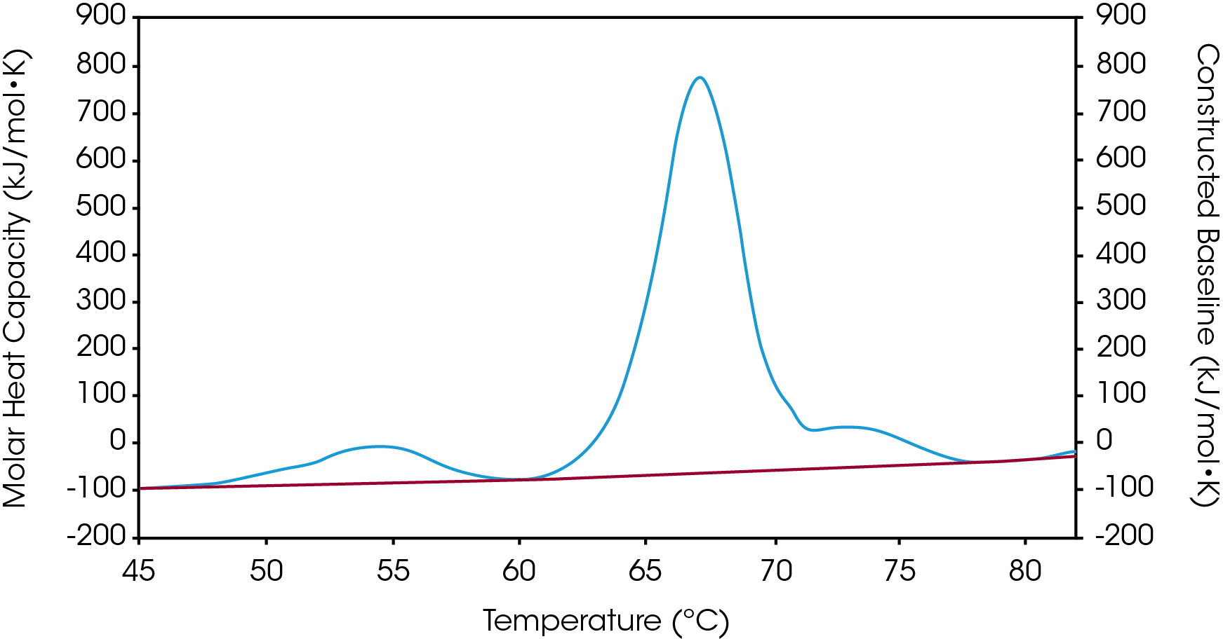
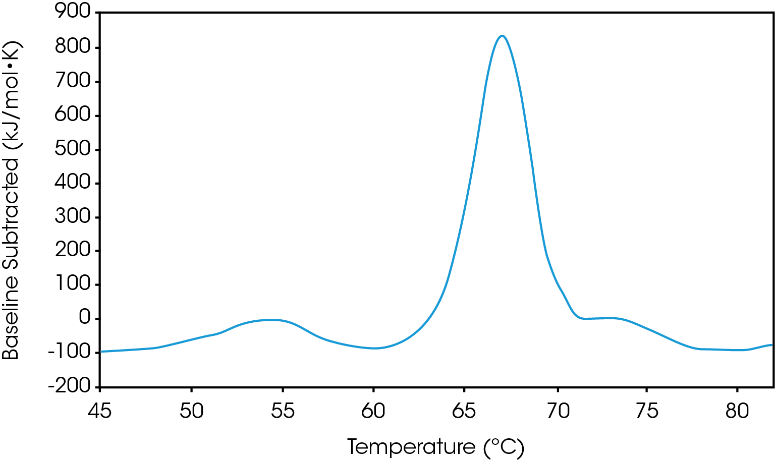
There are two baselines one could choose to use when analyzing DSC data, sigmoidal and polynomial. The sigmoidal baseline is applicable when analyzing a single two-state transition where a ΔCp is observed. When drawing the sigmoidal baseline, it is ideal to have around 10-15 °C of pre and post transitional baseline present, Figure 3. How the sigmoidal baseline is constructed is at the TM, the inflection point of the sigmoid is at the midpoint between the pre and post translational baselines. Additional points are made looking at % unfolded in relationship to the pre- and post-translational baselines. This is what ultimately leads to the “S” shape. Once subtracted, the pre- and post-transitional baselines will be zeroed, and modeling can be applied to determine the van’t Hoff enthalpy associated with the unfolding of the macromolecule.
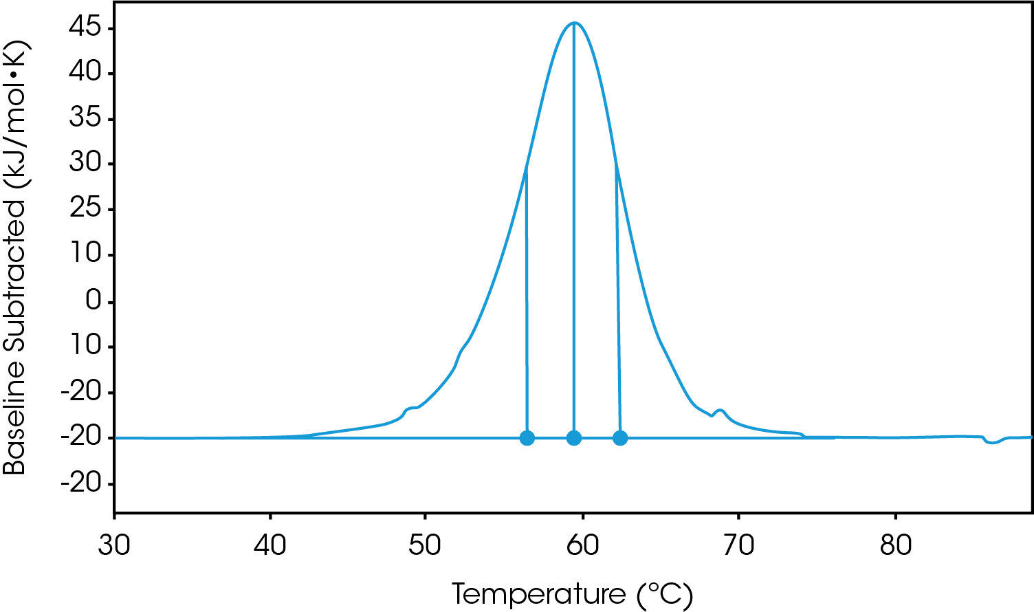
The polynomial baseline, Figure 4, should be used when there are multiple transitions present or when there is no observable ΔCp. The sigmoidal baseline will no longer apply when multiple transitions because a sigmoidal baseline would subtract out the total change in heat capacity of the system which is likely not the same for each individual transition. The other consideration is the construction of the baseline itself, as it would not be accurately drawn because each TM would not be used independently, but instead an average would be used. Therefore, a polynomial baseline will help obtain a more accurate value for ΔH of each transition during peak deconvolution.
Two-State / Two-State Scaled Model
The two-state model assumes the macromolecule to be either folded or unfolded (i.e. two states), and the van’t Hoff enthalpy is calculated based on the sharpness and shape of the unfolding peak.4 This model assumes that any concentration and MW information entered in the molar heat capacity conversion dialog to be accurate. If either of these quantities is off, then the modeled peak will not be able to simultaneously match both the width and height of the data peak.
The two-state scaled model adds a scaling factor (Aw) that compensates for errors in the assigned concentration. Such errors may arise from imprecise concentration determination or not knowing the precise oligomeric state of the sample. When using either the simple or scaled two-state model, the data must be baseline-subtracted. The correct baseline to apply is sigmoidal, which was discussed in the baseline section.
The two-state models can be used to confirm if a macromolecule truly unfolds in a two-state fashion as one will obtain a dHvH that is equal to the dHcal. If dHvH is less than dHcal this indicates the macromolecule unfolds through an intermediate state and the two-state model would not be valid. If dHvH is greater than dHcal this indicates the macromolecule is in an oligomeric state and two-state model can still be valid.5
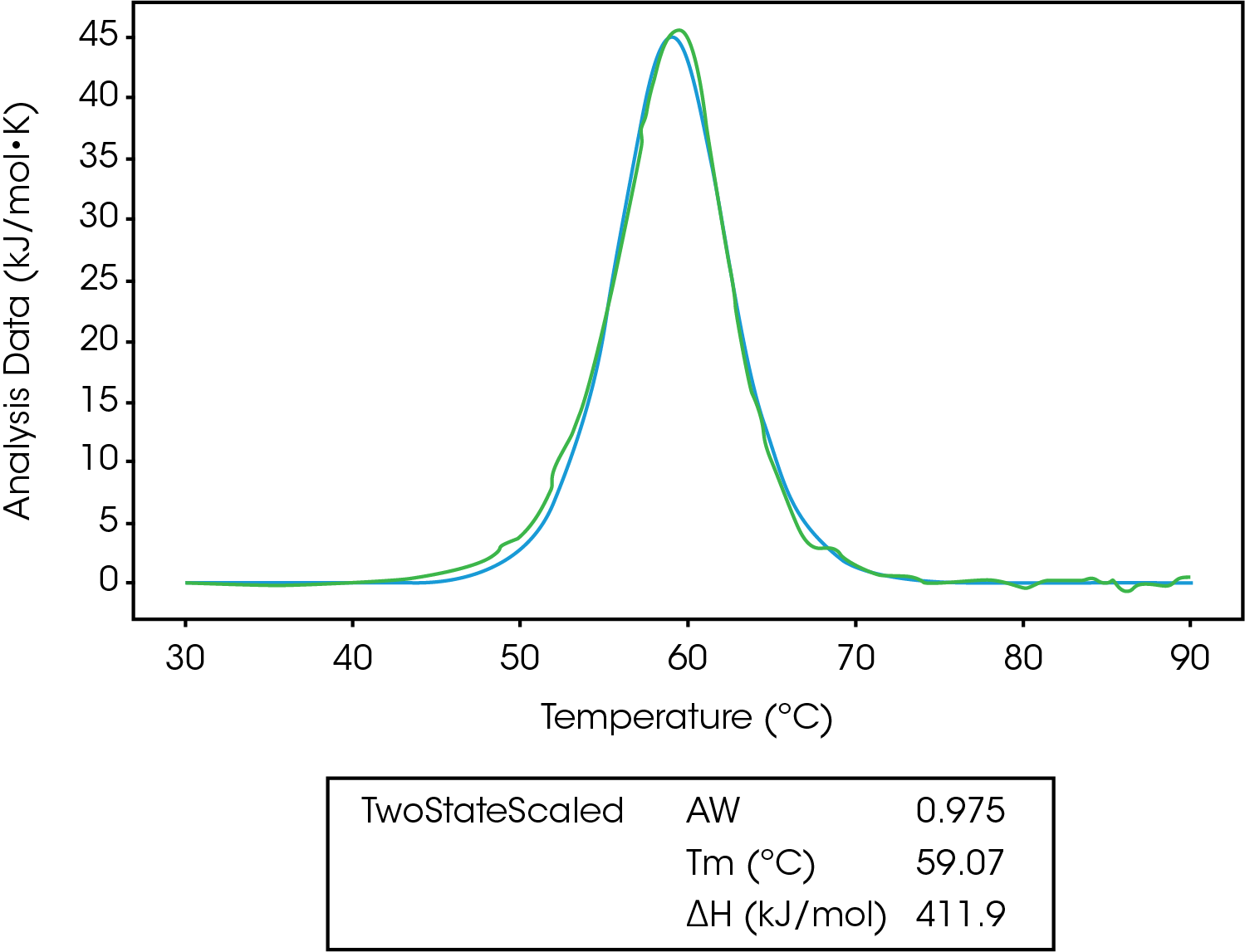
In Figure 5, we can see the unfolding of lysozyme fit to a two-state scaled model. The first thing to notice is the Aw factor is equal to 0.975, which means there is a slight error in concentration, and we likely don’t have 100% of the lysozyme starting in the native folded state. After taking this into account, ΔHcal is equal to ΔHvH, confirming a two-state transition.5
Gaussian/Gaussian with Tonset Model
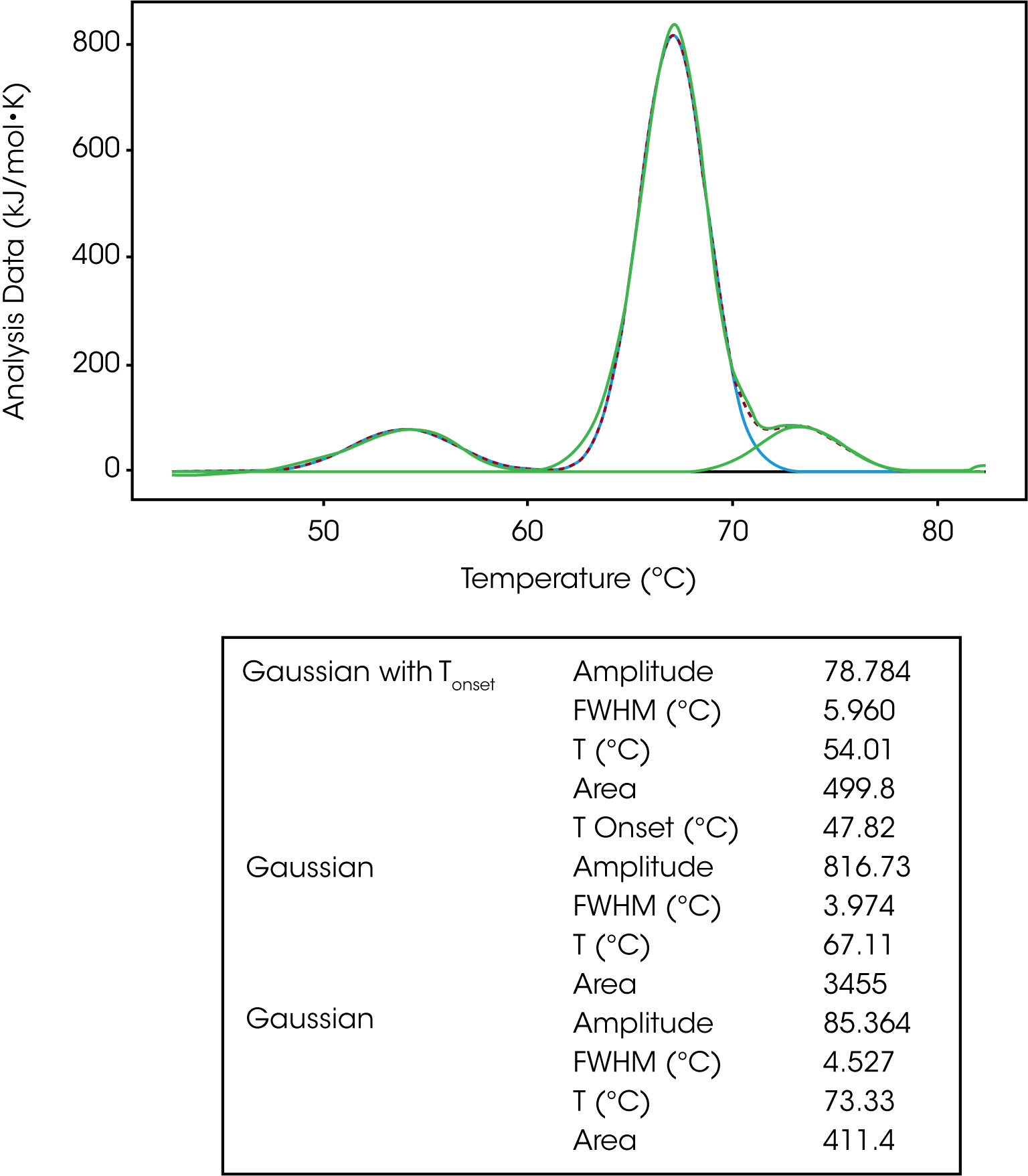
The Gaussian model is a generic model that mathematically describes the symmetric unfolding of a molecule, and it can be used when deconvoluting a multi-transition unfolding event. For example, IgG has three transitions and three models were fit to deconvolute the TM and enthalpy of each transition, Figure 4. As discussed in the baseline section, a polynomial baseline was constructed and subtracted from the data. The gaussian model provides information on the amplitude, FWHM, TM and enthalpy (area). If one were to choose the Gaussian with Tonset, the temperature of the onset of melting would also be determined.
In Figure 6, IgG was fit with one Gaussian Tonset model and two regular Gaussian models. Based on the Tonset, IgG starts to unfold at a temperature of 47.82 °C. There are three transitions with TMs of 54.01 °C, 67.11 °C and 73.33 °C. The second transition has the greatest enthalpy (3455 kJ/mol) and unfolds more cooperatively based on the lowest FWHM value of 3.974. There has been a lot of work done characterizing the unfolding of antibodies. It has been determined the first peak of an antibody thermogram is typically the CH2 domain and the largest peak is the Fab and the third is the CH3 domain.6-7
| Gaussian with Tonset | Amplitude | 78.784 |
|---|---|---|
| FWHM (°C) | 5.960 | |
| T (°C) | 54.01 | |
| Area | 499.8 | |
| T Onset (°C) | 47.82 | |
| Gaussian | Amplitude | 816.73 |
| FWHM (°C) | 3.974 | |
| T (°C) | 67.11 | |
| Area | 3455 | |
| Gaussian | Amplitude | 85.364 |
| FWHM (°C) | 4.527 | |
| T (°C) | 73.33 | |
| Area | 411.4 |
Voigt/ Voigt with Tonset Model
The Voigt model is a hybrid of a Gaussian and Lorentzian function. A Lorentzian peak has wider tails (outliers) than a Gaussian. So, given the same area under the peaks, the Lorentzian will be narrower than the Gaussian and with wider tails. For this reason, the Voigt model tends to fit DSC peaks better than the Gaussian function alone giving an enthalpy closer to the calorimetric enthalpy calculated in the NanoAnalyze Integration Baseline tab. For this reason, the Voigt model is great for peak deconvolution and for a single transition that isn’t a true two-state unfolding event. The same IgG data set was fit using three Voigt models. If we focus on the second transition, we can see the Voigt model does a better job of fitting the peak amplitude and tailing data thus calculating a more accurate ΔH value, Figure 7.
The same baseline guidance applies when fitting a multi-transition data set with a Voigt model. One should use a polynomial baseline and the onset temperature can be calculated by using the Voigt model with Tonset, shown in the modeling of the first transition in Figure 7.
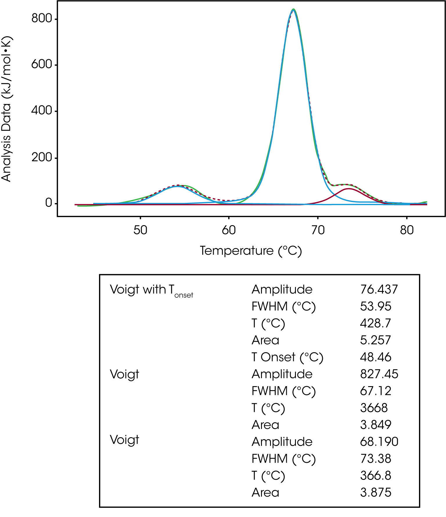
| Voigt with Tonset | Amplitude | 76.437 |
|---|---|---|
| FWHM (°C) | 53.95 | |
| T (°C) | 428.7 | |
| Area | 5.257 | |
| T Onset (°C) | 48.46 | |
| Voigt | Amplitude | 827.45 |
| FWHM (°C) | 67.12 | |
| T (°C) | 3668 | |
| Area | 3.849 | |
| Voigt | Amplitude | 68.190 |
| FWHM (°C) | 73.38 | |
| T (°C) | 366.8 | |
| Area | 3.875 |
Independent Non-Two State Model
The independent non-two state model is used to model systems that unfold through an intermediate state. If the van’t Hoff enthalpy of unfolding is smaller than the calorimetric enthalpy it is likely that intermediate states are formed during the unfolding process. So, this model could be used when a two-state model fails to fit the data properly. However, if there are intermediate states and asymmetrical unfolding, one might consider using a Voigt model or multiple Voigt models to deconvolute the unfolding as tailing data will likely be present.
General Model
The general model is the most complex in terms of variables to fit. This model is used to derive ΔCp from a model. Remember, the change in the heat capacity of a compound reflects its ability to absorb heat and experience a defined increase in temperature. It has been shown the sign of ΔCp distinguishes apolar (+) from polar (–) solvation. So, the solvation of polar groups found in proteins is characterized by a negative ΔCp.8-10 Also, globular protein unfolding usually has a positive ΔCp and when looking at stability versus temperature profile there is an inverted U-shape.8,9 This means proteins have a maximum stability and the downward U-shape implies that proteins become less stable at lower temperatures, which can lead to cold denaturation.8,9
The A0 and A1 variables of this model represent the intercept and slope of the leading baseline (before the transition), respectively. It is important to not subtract the baseline when fitting to this model, however, it is important to subtract the blank experiment (buffer/buffer). The baseline can’t be subtracted as the main function of this model is to determine the ΔCp, which is determined from the pre and post transitional baselines. In Figure 8, we see the unfolding of lysozyme fit with a general model.
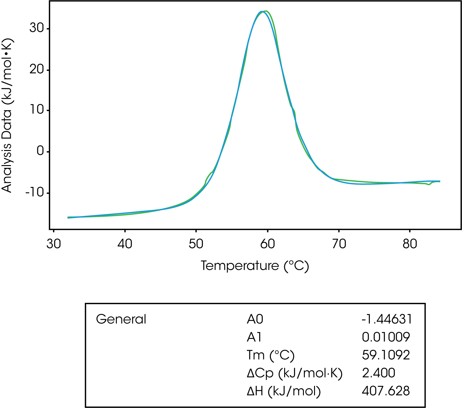
| General | A0 | -1.44631 |
|---|---|---|
| A1 | 0.01009 | |
| Tm (°C) | 59.1092 | |
| ΔCp (kJ/mol·K) | 2.400 | |
| ΔH (kJ/mol) | 407.628 |
Conclusions
In this application note, we discussed the general guidelines for the various models available in our NanoAnalyze software to be used for analyzing thermograms, and what to consider when selecting a specific model.
1. Bruylants, G., Wouters, J., Michaux C “Differential scanning calorimeter in life sciences: thermodynamics, stability, molecular recognition, and applications in drug design” Curr. Med. Chem (2005) 12: 2011-2020
2. Freire, E “Thermal denaturation methods in the study of protein folding” Methods Enzymol (1995) 259: 144-168
3. Shindoa, K “Iceberg formation and solubility” J. Phys. Chem (1977) 81: 8069-8072
4. Privalov, P.L and Potekhin “Scanning Microcalorimetry in Studying Temperature Induced Changes in Proteins” Methods in Enzymology (1986) 141:4-51
5. Marky, L.A., Breslauer K.J. “Calculating thermodynamic data for transitions of any molecularity from equilibrium melting curves” Biopolymers (1987) 26: 1601-1620
6. Garber, E., Demarest, S.J. “A Broad Range of Fab Stabilities within a Host of Therapeutic IgGs” Biochem. Biophys. Res. Commun. (2007) 355: 751–757
7. Ionsecu, R., Vlasak, J.; Price, C., Kirchmeier, M. “Contribution of Variable Domains to the Stability of Humanized IgG1 Monoclonal Antibodies” Journal of Pharmaceutical Sciences (2008) 97(4): 1414-1426
8. Prabhu, N.V., and Sharp, K.A. “Heat Capacity in Proteins” Annu. Rev. Phys Chem (2005) 56: 521-48
9. Privalov, P.L., and Gill S.J. “ Stability of Protein Structure and Hydrophobic Interaction” Adv. Prot. Chem. (1988) 39:191–234
10. Makhatadze GI, Privalov PL. “ Heat capacity of proteins: I. Partial molar heat capacity of individual amino acid residues in aqueous solution: Hydration effect” J. Mol. Biol. (1990) 213:375–84
Acknowledgement
This application note was written by Calliste Scholl, Applications Engineer at TA Instruments.
Click here to download the printable version of this application note.

